Outliers can be evaluated once the required data are successfully imported into R (see the data input and checks vignette for an overview). The results data file with the monitoring data is required. The data quality objectives file for accuracy is also required to determine plot axis scaling as arithmetic (linear) or logarithmic and to fill results data that are below detection or above quantitation limits. The example data included with the package are imported here to demonstrate how to use the analysis functions:
library(MassWateR)

# import results data
respth <- system.file("extdata/ExampleResults.xlsx", package = "MassWateR")
resdat <- readMWRresults(respth)
#> Running checks on results data...
#>  Checking column names... OK
#>  Checking all required columns are present... OK
#>  Checking valid Activity Types... OK
#>  Checking Activity Start Date formats... OK
#>  Checking depth data present... OK
#>  Checking for non-numeric values in Activity Depth/Height Measure... OK
#>  Checking Activity Depth/Height Unit... OK
#>  Checking Activity Relative Depth Name formats... OK
#>  Checking values in Activity Depth/Height Measure > 1 m / 3.3 ft... OK
#>  Checking Characteristic Name formats... OK
#>  Checking Result Values... OK
#>  Checking for non-numeric values in Quantitation Limit... OK
#>  Checking QC Reference Values... OK
#>  Checking for missing entries for Result Unit... OK
#>  Checking if more than one unit per Characteristic Name... OK
#>  Checking acceptable units for each entry in Characteristic Name... OK
#>
#> All checks passed!

# import accuracy data
accpth <- system.file("extdata/ExampleDQOAccuracy.xlsx", package = "MassWateR")
accdat <- readMWRacc(accpth)
#> Running checks on data quality objectives for accuracy...
#>  Checking column names... OK
#>  Checking all required columns are present... OK
#>  Checking column types... OK
#>  Checking no "na" in Value Range... OK
#>  Checking for text other than <=, ≤, <, >=, ≥, >, ±, %, AQL, BQL, log, or all... OK
#>  Checking overlaps in Value Range... OK
#>  Checking gaps in Value Range... OK
#>  Checking Parameter formats... OK
#>  Checking for missing entries for unit (uom)... OK
#>  Checking if more than one unit (uom) per Parameter... OK
#>  Checking acceptable units (uom) for each entry in Parameter... OK
#>  Checking empty columns... OK
#>
#> All checks passed!
Analyzing outliers
Outliers can be identified using the anlzMWRoutlier()
function. Evaluating data for outliers is a critical step of quality
control, and this function allows a user to quickly identify them for
removal or additional follow-up. Outliers are defined using the standard
definition of 1.5 times the interquartile range (the 25th to 75th
percentile) of a parameter, depending on the grouping used for the
function. They are visually identified as points above or below the
whiskers in the boxplots that describe distribution of the data, i.e.,
the box defines the interquartile range, the horizontal line is the
median, and the whiskers extend above and below 1.5 times the
interquartile range.
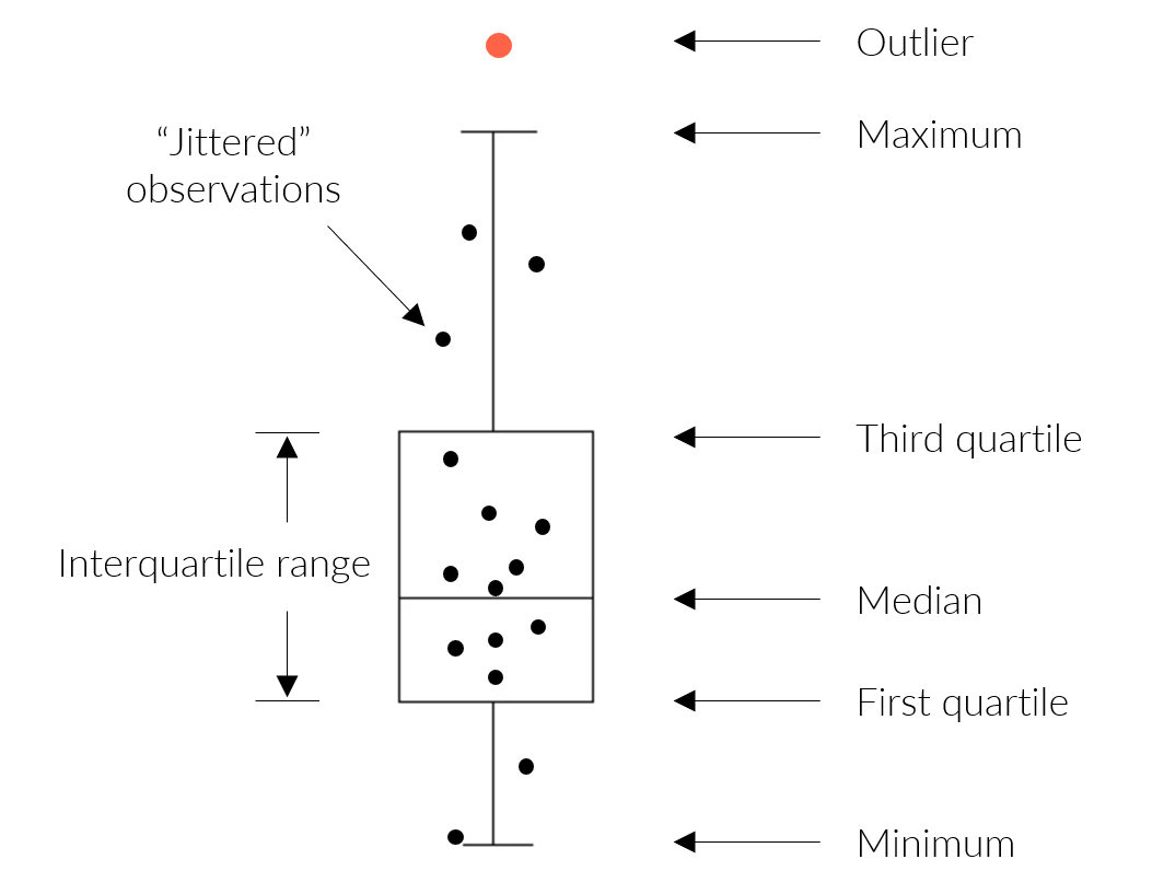
A summary of the distribution statistics shown with a standard boxplot. Outliers extend beyond the whiskers and are 1.5 times the interquartile range.
The anlzMWRoutlier() function uses the results data as a
file path or data frame as input. The data quality objectives for
accuracy is also required. The input files are passed to the function
using the res and acc arguments, but a named
list with the same arguments can also be used with the fset
argument for convenience. The results for a selected parameter are shown
as boxplots, with the outliers labelled accordingly.
anlzMWRoutlier(res = resdat, param = "DO", acc = accdat, group = "month")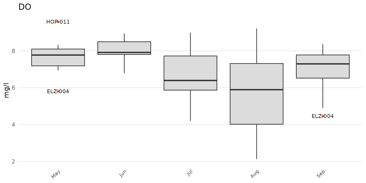
Outliers can be shown by month using group = "month", by
site using group = "site", or by week of year using
group = "week". Above, outliers are shown for dissolved
oxygen grouped by month. The same data can also grouped by site.
anlzMWRoutlier(res = resdat, param = "DO", acc = accdat, group = "site")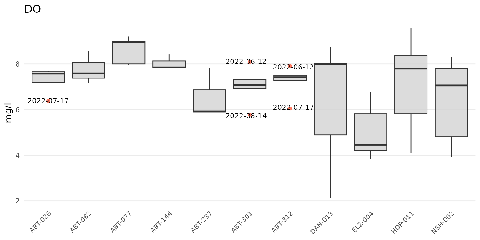
The same data can also be grouped by week using
group = "week". The week of the year is shown on the plot
as an integer. Note that there can be no common month/day indicating the
start of the week between years and an integer is the only way to
compare summaries if the results data span multiple years.
anlzMWRoutlier(res = resdat, param = "DO", acc = accdat, group = "week")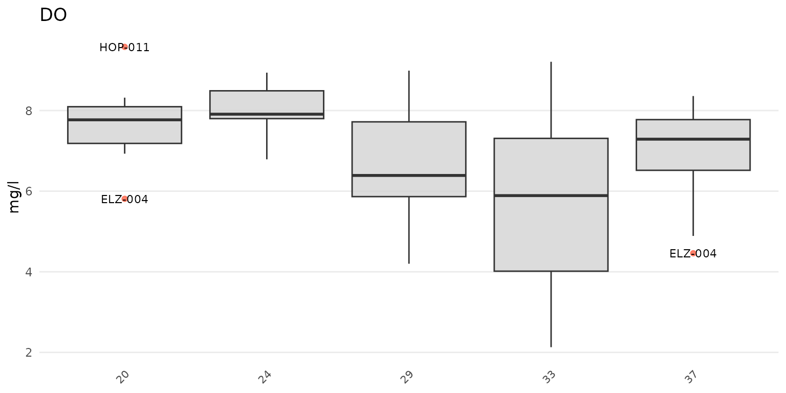
Results can also be filtered by dates using the dtrng
argument. The date format must be YYYY-MM-DD and include
two entries.
anlzMWRoutlier(res = resdat, param = "DO", acc = accdat, group = "week", dtrng = c("2022-05-01", "2022-07-31"))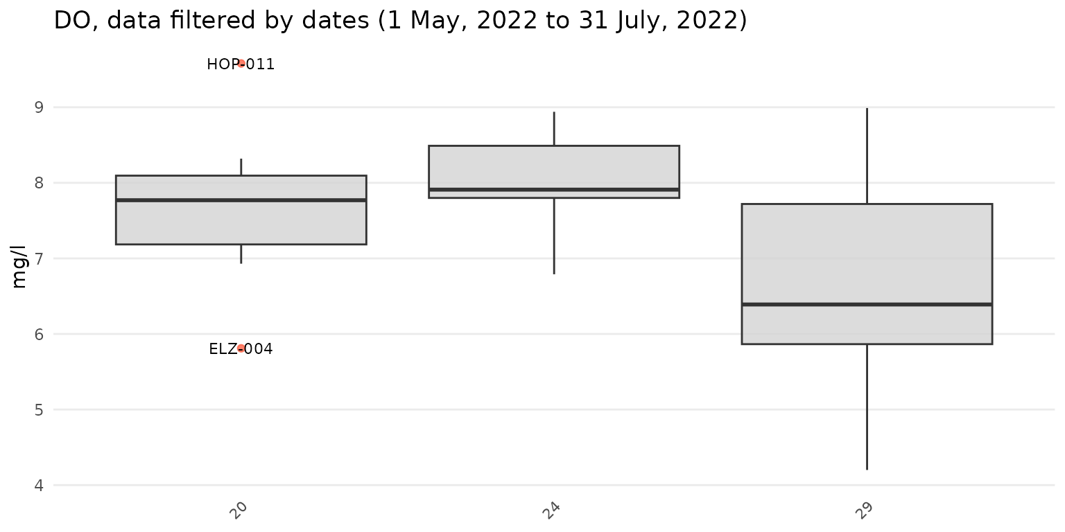
Points that are not outliers can also be jittered over the boxplots
using type = "jitterbox" (default is
type = "box"). Outlier labels that overlap are also offset
by default. This can be suppressed using repel = FALSE.
anlzMWRoutlier(res = resdat, param = "DO", acc = accdat, type = "jitterbox", group = "month", repel = FALSE)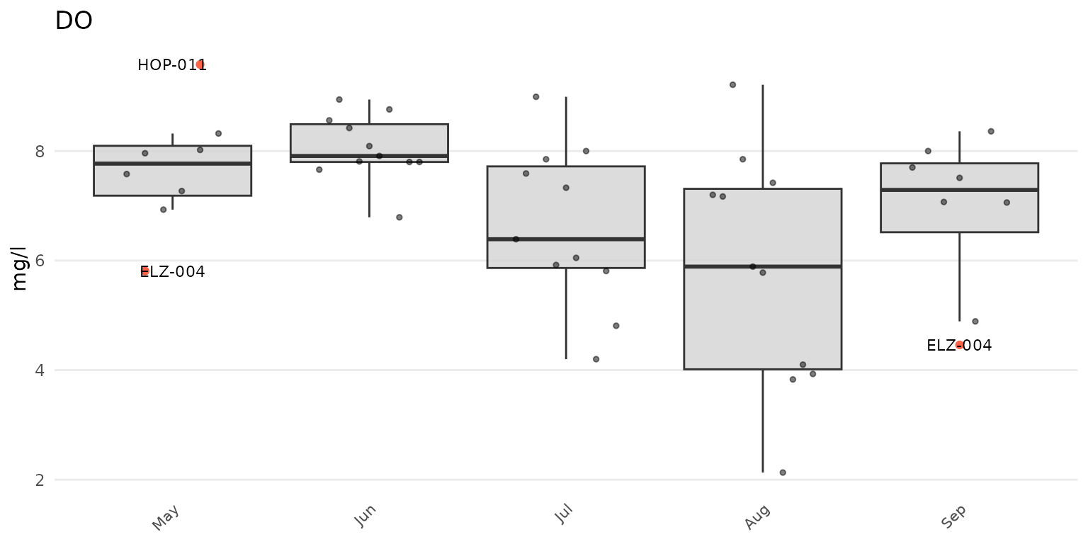
Specifying type = "jitter will suppress the
boxplots.
anlzMWRoutlier(res = resdat, param = "DO", acc = accdat, type = "jitter", group = "month")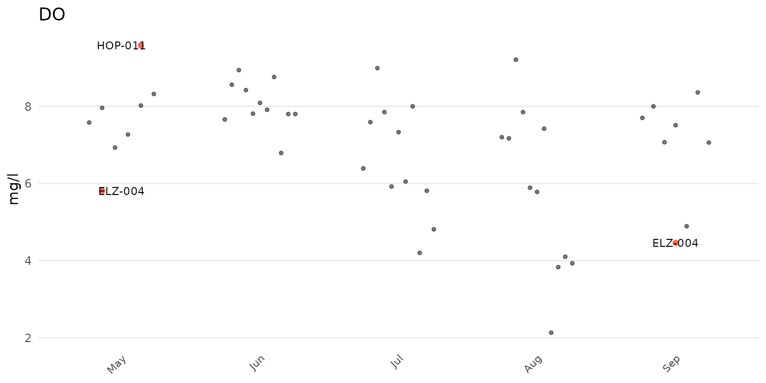
The y-axis scaling as arithmetic (linear) or logarithmic can be set
with the yscl argument. If yscl = "auto"
(default), the scaling is determined automatically from the data quality
objective file for accuracy, i.e., parameters with “log” in any of the
columns are plotted on log10-scale, otherwise arithmetic. Setting
yscl = "linear" or yscl = "log" will set the
axis as linear or log10-scale, respectively, regardless of the
information in the data quality objective file for accuracy. Below, the
axis for E. Coli is plotted on the log-10 scale automatically. The
y-axis scaling does not need to specified explicitly in the function
call because the default setting is yscl = "auto".
anlzMWRoutlier(res = resdat, param = "E.coli", acc = accdat, group = "site")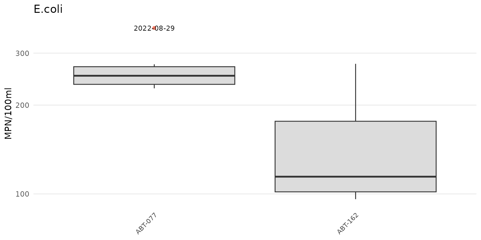
To force the y-axis as linear for E. Coli,
yscl = "linear" must be used. Note that the default linear
scaling for dissolved oxygen above is determined automatically.
anlzMWRoutlier(res = resdat, param = "E.coli", acc = accdat, group = "site", yscl = "linear")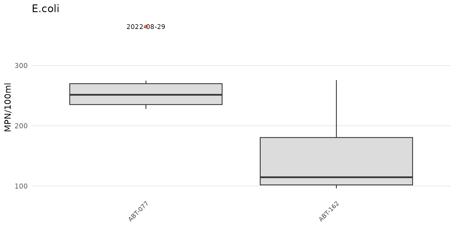
Finally, a data frame of the identified outliers can also be returned
by setting outliers = TRUE. This table can be used to
identify the outliers in the original data for removal or additional
follow-up.
anlzMWRoutlier(res = resdat, param = "DO", acc = accdat, group = "month", outliers = TRUE)
#> # A tibble: 3 × 6
#>   `Monitoring Location ID` `Activity Start Date` `Activity Start Time`
#>   <chr>                    <dttm>                <chr>
#> 1 ELZ-004                  2022-05-15 00:00:00   06:50
#> 2 HOP-011                  2022-05-15 00:00:00   06:55
#> 3 ELZ-004                  2022-09-11 00:00:00   07:20
#> # ℹ 3 more variables: `Characteristic Name` <chr>, `Result Value` <dbl>,
#> #   `Result Unit` <chr>
Output all outlier results
Outlier plots for all parameters in the results data file can be
created using the anlzMWRoutlierall() function. This can be
used to create a word document with all plots embedded in the file or as
separate png images saved to a specified directory. The relevant
arguments required for the function include format = "word"
or format = "png" to specify the output type,
fig_height and fig_width for the plot
dimensions (default as 4 and 8, respectively), and
output_dir and output_file for the output
directory and file name. The rest of the arguments are all those
required for anlzMWRoutlier(), except the
param argument because plots for all parameters are created
in the output.
Create a word document for all outlier plots in a temporary directory:
anlzMWRoutlierall(res = resdat, acc = accdat, group = 'month', format = 'word', output_dir = tempdir())Create the same output but as separate png plots for each parameter:
anlzMWRoutlierall(res = resdat, acc = accdat, group = 'month', format = 'png', output_dir = tempdir())The inputs can also be passed to the fset argument as a
named list for convenience.
# names list of inputs
fsetls <- list(
  res = resdat,
  acc = accdat
)

anlzMWRoutlierall(fset = fsetls, group = 'month', format = 'word', output_dir = tempdir())
Once the function is done running, a message indicating success and where the file(s) is located is returned.